
Tommy's Blog
Reinforcement Learning
Introduction
The purpose of this post is to explain the core concept behind reinforcement learning (RL). It was written for people that already understand supervised learning (SL) and want to start exploring RL. To build our intuition, we’ll train a model on a simplified version of the next token prediction task used to train LLMs. Through this toy problem we’ll learn about RL concepts like reward shaping, exploration and how to tune these parameters to get good results. We’ll also train a hybrid model (SL pre-train + RL fine-tune) and see how it significantly outperforms training with SL or RL alone.
If you would prefer to read through this post interactively and run the code here’s a notebook.
Ok, so what’s the core idea that makes RL different to SL?
Learning Strategies
Humans use different strategies to acquire knowledge and skills. Two of the most well known strategies are:
- Imitation: watch someone do a task and copy them
- Trial and Error: do the task yourself and learn based on what happens
In machine learning we have analogous strategies:
- Supervised Learning (SL): learn by imitating examples
- Reinforcement Learning (RL): learn through trial and error
To see how these strategies differ in practice, let’s consider a toy version of the next token prediction task used to train LLMs. In the real task, a model takes a sequence of tokens as input and predicts the next token from thousands of options, such that the total sequence satisfies some higher-level criteria like helpfulness or accuracy.
In our simplified version, the model takes a 3-digit number as input (e.g. [4,3,3]), and it must predict 2 more digits such that all 5 digits sum to 20. For the input [4,3,3], valid predictions would include [7,3], [1,9], [6,4] or any pair that brings the total to 20.
Later in the post we’ll be training a model to solve this 3+2 problem. To build our intuition, let’s begin with an even simpler version where the model takes 4 digits as input and must output a single digit to complete the sequence. This lets us focus on the mechanics of a single prediction.
What does each strategy look like for this problem? Both approaches train a model that outputs a probability distribution for the digits 0 to 9. The difference is in how the model learns to shape that distribution:
- SL: The distribution is shaped by imitating training labels. Given
[4,3,3,7]with label3, the model learns to increase the probability of outputting3. - RL: The distribution is shaped through trial and error. The model samples from its own distribution, and when it stumbles upon a correct answer (5 digits summing to 20), it updates the model to make that output more likely.
Ok, what do these strategies look like in code?
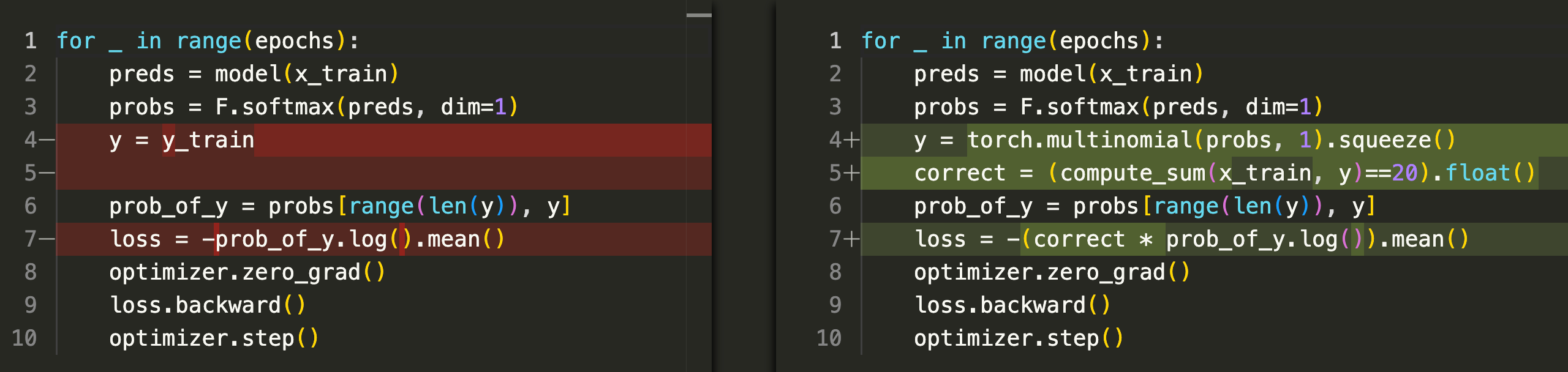
As we can see the basic mechanics are the same. We feed the training data through our model, we generate a probability distribution, compute our loss and update the model weights using back propagation. The key difference lies in how the loss is generated.
In SL, the loss is standard cross-entropy loss (i.e. the negative log probability of the training labels y). In RL, we don’t have labels. Instead, on line 4 we sample from the model’s own probability distribution to generate outputs. On line 5 we check if these outputs are correct by seeing if the sum of inputs + outputs is 20. The loss is then the same cross-entropy loss used in SL, except we use the correct vector to prevent any incorrect solutions from impacting the model’s weights during backpropagation. This means that the model only learns from valid outputs.
The correct vector above is usually called a reward. Why do we use the term reward?
The term reward comes from behavioural psychology where rewards are given to help encourage or reinforce certain behaviours. In RL, the behaviour we want to reinforce is the generation of valid outputs. That’s why we only reward the model when it generates valid outputs.
Now that we have a little intuition, let’s go ahead and train a model with RL. We’ll start with the basic RL training loop shown above and we’ll improve it step-by-step until we match the results of an SL trained model.
The Problem
As mentioned above we’re going to train a model that takes 3 digits as input and outputs 2 digits such that the 5 digits sum to 20.
Before we get started let’s create a little helper function to make reproducibility easier. The results are quite sensitive to this seed so we’ll run it everytime we train a model or use the random module.
Note: Even with a fixed seed, results may vary across different hardware.
# !pip install torch
import random
import torch
import torch.nn as nn
import torch.nn.functional as F
from functools import partial
def set_seed(seed=-1): random.seed(seed); torch.manual_seed(seed)
Setup
Data
First let’s build our dataset of input/output pairs.
def make_data():
    data = []
    for input_ in range(1_000):
        for output_ in range(100):
            d1,d2,d3 = [int(o) for o in str(input_).zfill(3)]
            d4,d5 = divmod(output_,10)
            if d1+d2+d3+d4+d5 == 20: data.append([d1,d2,d3,d4,d5])
    return data
data = make_data()
This gives us 5,631 examples like the ones below:
[0, 2, 4, 6, 8][1, 5, 8, 5, 1][4, 4, 4, 4, 4]
Validation Set
Now we need to split our data into training and validation sets. We could just randomly split the data, but a more stringent test would be splitting on the 3-digit inputs the model receives. We have 912 unique inputs (e.g. [0, 2, 4]). We’ll include 80% of these inputs in our training dataset and use the remainder in the validation set.
def split_data(data):
    set_seed()
    inputs = list(set((d1,d2,d3) for d1,d2,d3,*_ in data))
    random.shuffle(inputs)
    split = int(0.8*len(inputs))
    train_inputs = set(inputs[:split])
    train_data = [row for row in data if tuple(row[:3]) in train_inputs]
    val_data = [row for row in data if tuple(row[:3]) not in train_inputs]
    return train_data, val_data
train, val = split_data(data)
Input Encoding
We could pass our inputs (e.g. [0, 2, 4]) directly to the model. Another approach is to use one-hot encoding, where each digit becomes a 10-dimensional binary vector (e.g., 3 → [0,0,0,1,0,0,0,0,0,0]). Since we have 3 input digits, we would concatenate each 10-dim vector to get a 30-dim input vector. One-hot encoding produced better results, so we’ll use that.
Output Format
What about the output? We could have our model predict two separate digits e.g. [2, 4] or make it autoregressive and use 2 forward passes. To keep things as simple as possible, let’s merge the two output digits into a single number (e.g. [6,8] → 68). This means our model will now output a 100-dim vector. If our model receives an input of [0, 2, 4], then our model should learn to assign a large probability to the 68th element of the 100-dim vector (which represents [6,8]) or any other valid output like the 77th element [7,7].
Now that we’ve decided on the structure of our dataset we need to convert it to tensors. The torchify function below takes our list of 5-digit numbers, one-hot encodes the input, and creates the merged output we discussed above.
def torchify(data):
    X = torch.tensor([[d1,d2,d3] for d1,d2,d3,*_ in data])
    Y = torch.tensor([[d4,d5] for *_,d4,d5 in data])
    X_onehot = torch.cat([F.one_hot(X[:,0], 10), F.one_hot(X[:,1], 10), F.one_hot(X[:,2], 10)], dim=1).float()
    Y_combined = Y[:, 0]*10 + Y[:, 1]
    return X_onehot, Y_combined
x_train, y_train = torchify(train)
x_val, y_val = torchify(val)
Model
Now we’re ready to define our model. We’re going to use a multi-layer perceptron (MLP) with one hidden layer of 64 neurons. It takes a 30-dim input and outputs a 100-dim vector. We could have used a larger model, but I thought it would be a fun challenge to work with something so tiny.
def _model(): return nn.Sequential(nn.Linear(30, 64), nn.ReLU(), nn.Linear(64, 100))
Training
Finally, we’re ready to train our model. We’re going to train 3 versions of the model. An SL version, an RL one and finally an SL/RL hybrid.
Our goal is to reach 90% accuracy on the validation set in 10k epochs or less.
⚠️ We want to keep our training loop as simple as possible. This means we’ll forgo many best practices like mini-batch training, cyclical learning rates, etc. ⚠️
n_epochs = 10_000
Supervised Learning
Let’s create a basic SL training loop.
def train_sl(x_train, y_train, x_val, y_val, lr=0.01):
    set_seed()
    model = nn.Sequential(nn.Linear(30, 64), nn.ReLU(), nn.Linear(64, 100))
    optimizer = torch.optim.Adam(model.parameters(), lr=lr)
    for epoch in range(epochs):
        out = model(x_train)
        loss = F.cross_entropy(out, y_train)
        optimizer.zero_grad()
        loss.backward()
        optimizer.step()
        if epoch % 1000 == 0 or epoch == epochs-1:
            with torch.no_grad(): val_loss = F.cross_entropy(model(x_val), y_val)
            if epoch == 0:
                print("| Epoch | Train Loss | Val Loss |")
                print("|-------|------------|----------|")
            print(f"| {epoch:5d} | {loss:10.4f} | {val_loss:8.4f} |")
    return model
Before running it, let’s make it more modular as that will allow us to experiment faster.
def train_sl(model, opt, loss_fn, logger_fn, x_train, y_train, x_val, y_val, epochs=n_epochs):
    for epoch in range(epochs):
        preds = model(x_train)
        loss = loss_fn(preds, y_train)
        opt.zero_grad()
        loss.backward()
        opt.step()
        logger_fn(model, loss_fn, loss, x_val, y_val, epoch, epochs)
    return model
def logger(model, loss_fn, train_loss, x_val, y_val, epoch, total_epochs):
    if epoch % 1000 != 0 and epoch != total_epochs-1: return
    with torch.no_grad(): val_loss = loss_fn(model(x_val), y_val)
    if epoch == 0:
        print("| Epoch | Train Loss | Val Loss |")
        print("|-------|------------|----------|")
    print(f"| {epoch:5d} | {train_loss:10.4f} | {val_loss:8.4f} |")
Ok, let’s run it.
set_seed()
model = _model()
opt = torch.optim.Adam(model.parameters(), lr=0.01)
sl_loss = F.cross_entropy
model_sl = train_sl(model, opt, sl_loss, logger, x_train, y_train, x_val, y_val)
| Epoch | Train Loss | Val Loss |
|---|---|---|
| 0 | 4.6133 | 4.6015 |
| 1000 | 1.9267 | 5.8485 |
| 2000 | 1.9234 | 6.5603 |
| 3000 | 1.9229 | 6.9767 |
| 4000 | 1.9226 | 7.2907 |
| 5000 | 1.9217 | 7.5535 |
| 6000 | 1.9215 | 7.8406 |
| 7000 | 1.9212 | 8.0942 |
| 8000 | 1.9211 | 8.2726 |
| 9000 | 1.9211 | 8.4537 |
| 9999 | 1.9218 | 8.7833 |
Yikes! Our validation loss is diverging from our training loss so we’re clearly overfitting. Let’s add some weight decay to see if that helps.
set_seed()
model = _model()
opt = torch.optim.Adam(model.parameters(), lr=0.01, weight_decay=0.001)
model_sl = train_sl(model, opt, sl_loss, logger, x_train, y_train, x_val, y_val)
| Epoch | Train Loss | Val Loss |
|---|---|---|
| 0 | 4.6133 | 4.6015 |
| 1000 | 2.5367 | 2.8668 |
| 2000 | 2.5338 | 2.8742 |
| 3000 | 2.4434 | 2.7471 |
| 4000 | 2.3318 | 2.5231 |
| 5000 | 2.3309 | 2.5283 |
| 6000 | 2.3307 | 2.5275 |
| 7000 | 2.3307 | 2.5274 |
| 8000 | 2.3309 | 2.5275 |
| 9000 | 2.3306 | 2.5270 |
| 9999 | 2.3295 | 2.5385 |
That looks much better but what about accuracy on the validation set?
To check this let’s create a function test_model that takes all the unique prefixes in our validation set, runs them through our model and computes the % that sum to 20.
To compute the sum we’ll need to convert our 1-hot encoded inputs back to digits (e.g. [0,0,0,1,0,0,0,0,0,0] => 3).
def onehot2digits(x): return x.view(-1, 3, 10).argmax(dim=2).T
Now, let’s build a method that computes accuracy.
def _accuracy(model, x):
    with torch.no_grad(): preds = model(x).argmax(dim=1)
    d1,d2,d3 = onehot2digits(x)
    d4,d5 = preds//10, preds%10
    return (d1+d2+d3+d4+d5 == 20).float().mean()
def test_model(model, x):
    x, _ = torch.unique(x, dim=0, return_inverse=True)
    print(f"Accuracy: {_accuracy(model, x):.2%}")
Ok, let’s check our accuracy.
test_model(model_sl, x_val)
Accuracy: 91.26%
Great. We’ve already hit our target of getting 90% accuracy on the validation set 🎉. Let’s move on to the RL training loop.
Reinforcement Learning
Let’s implement the basic RL training loop we saw in the Learning Strategies section. We’ll use the same modular approach as SL. All we need to do is to define a custom RL loss function.
def train_rl(model, opt, loss_fn, logger_fn, x_train, x_val, epochs=n_epochs):
    for epoch in range(epochs):
        preds = model(x_train)
        loss = loss_fn(preds, x_train)
        opt.zero_grad()
        loss.backward()
        opt.step()
        logger_fn(model, x_train, x_val, epoch, epochs)
    return model
Recall from the learning strategies section that computing the rl loss involves the following steps:
- converting the model’s predictions to a probability distribution
- sampling from the distribution
- checking if the sum of inputs + sampled outputs equals 20 and creating a corresponding reward vector
- computing the negative log probability of the sampled outputs
- use the reward vector as a filter so that the model only learns from valid solutions
def rl_loss_fn(preds, x):
    probs = F.softmax(preds, dim=1)
    y = torch.multinomial(probs, 1).squeeze()
    prob_of_y = probs[range(len(y)), y]
    d1,d2,d3 = onehot2digits(x)
    d4,d5 = y//10, y%10
    sums = d1+d2+d3+d4+d5
    rewards = (sums == 20).float()
    return -(rewards*prob_of_y.log()).mean()
PyTorch’s F.log_softmax has better numerical stability than calling .log on F.softmax. Let’s use that instead. We’ll sacrifice a little readability but that’s ok.
def rl_loss_fn(preds, x):
    log_probs = F.log_softmax(preds, dim=1)
    probs = torch.exp(log_probs)
    y = torch.multinomial(probs, 1).squeeze()
    log_prob_of_y = log_probs[range(len(y)), y]
    d1,d2,d3 = onehot2digits(x)
    d4,d5 = y//10, y%10
    sums = d1+d2+d3+d4+d5
    rewards = (sums == 20).float()
    return -(rewards*log_prob_of_y).mean()
We also need to build a custom rl logger because loss isn’t a useful measure of training progress in RL like it is in SL. Let’s print the training and validation accuracy instead.
def rl_logger(model, x_train, x_val, epoch, total_epochs):
    if epoch % 1000 != 0 and epoch != total_epochs-1: return
    x_train, _ = torch.unique(x_train, dim=0, return_inverse=True)
    x_val, _ = torch.unique(x_val, dim=0, return_inverse=True)
    train_acc, val_acc = _accuracy(model, x_train), _accuracy(model, x_val)
    if epoch == 0:
        print("| Epoch | Train Acc | Val Acc |")
        print("|-------|-----------|---------|")
    print(f"| {epoch:5d} | {train_acc:9.2%} | {val_acc:7.2%} |")
Let’s run it.
set_seed()
model = _model()
opt = torch.optim.Adam(model.parameters(), lr=0.015)
model_rl = train_rl(model, opt, rl_loss_fn, rl_logger, x_train, x_val)
| Epoch | Train Acc | Val Acc |
|---|---|---|
| 0 | 8.50% | 6.56% |
| 1000 | 24.14% | 12.02% |
| 2000 | 24.55% | 13.66% |
| 3000 | 24.69% | 14.75% |
| 4000 | 24.69% | 14.75% |
| 5000 | 24.69% | 14.75% |
| 6000 | 24.69% | 14.75% |
| 7000 | 24.69% | 14.75% |
| 8000 | 30.18% | 18.58% |
| 9000 | 30.32% | 18.58% |
| 9999 | 30.32% | 18.03% |
Yikes! The training and validation accuracy are terrible. Let’s take a look at what the model is predicting for a subset of the validation set.
def show_predictions(model, x, n=10):
    set_seed()
    x, _ = torch.unique(x, dim=0, return_inverse=True)
    idx = torch.randperm(len(x))[:n]
    x = x[idx]
    with torch.no_grad(): preds = model(x).argmax(dim=1)
    d1,d2,d3 = onehot2digits(x)
    d4,d5 = preds//10, preds%10
    sums = d1+d2+d3+d4+d5
    print("|  Input  | Output | Sum | Correct  |")
    print("|---------|--------|-----|----------|")
    for i in range(n):
        correct = "✅" if sums[i] == 20 else "❌"
        print(f"| [{d1[i]},{d2[i]},{d3[i]}] | [{d4[i]},{d5[i]}]  | {sums[i]:3} |    {correct}    |")
    print(f"\nUnique Outputs: {len(set(preds.tolist()))}")
show_predictions(model_rl, x_val)
| Input | Output | Sum | Correct |
|---|---|---|---|
| [0,5,0] | [2,9] | 16 | ❌ |
| [4,0,9] | [2,6] | 21 | ❌ |
| [2,8,9] | [4,3] | 26 | ❌ |
| [1,0,2] | [2,9] | 14 | ❌ |
| [8,4,0] | [2,6] | 20 | ✅ |
| [5,3,0] | [2,9] | 19 | ❌ |
| [1,4,2] | [2,9] | 18 | ❌ |
| [3,9,4] | [4,3] | 23 | ❌ |
| [4,0,2] | [2,9] | 17 | ❌ |
| [4,7,7] | [4,3] | 25 | ❌ |
Unique Outputs: 3
We can clearly see that the model is only generating a small subset of possible outputs. In this case only 3 unique outputs were generated. This phenomenon is known as mode collapse (mode in this context refers to a peak in the probability distribution). Why does this happen? Recall that our basic RL loop only learns when it generates a valid output. Early on, almost all outputs are incorrect. When the model stumbles into a valid solution it updates the model’s weights to make that output more likely to be sampled in the future. Like a doting parent it only sees when the output is successful and can’t see all the failures. As this output is being sampled more often, it gets more chances to be correct and thus more chances to update the model’s weights, making it even more likely to be sampled. This feedback loop results in the model generating a highly concentrated probability distribution where only a handful of outputs are sampled.
To counteract this problem we need to figure out how to encourage the model to make probs less concentrated.
Exploration
A common way of making probs less concentrated is by adding another term to our loss that penalises the model when probs is too concentrated. We can compute the concentration of probs by calculating it’s entropy. A distribution’s entropy is higher when it is more uniform and lower when it is more concentrated. Let’s update rl_loss and see if it helps.
def rl_loss_fn(preds, x, entropy_weight=0.1):
    log_probs = F.log_softmax(preds, dim=1)
    probs = torch.exp(log_probs)
    y = torch.multinomial(probs, 1).squeeze()
    log_prob_of_y = log_probs[range(len(y)), y]
    d1,d2,d3 = onehot2digits(x)
    d4,d5 = y//10, y%10
    sums = d1+d2+d3+d4+d5
    rewards = (sums == 20).float()
    entropy = -(probs*log_probs).sum(dim=1).mean()
    return -(rewards*log_prob_of_y).mean() - entropy_weight*entropy
set_seed()
model = _model()
opt = torch.optim.Adam(model.parameters(), lr=0.015)
rl_loss = partial(rl_loss_fn, entropy_weight=0.15)
model_rl = train_rl(model, opt, rl_loss, rl_logger, x_train, x_val)
| Epoch | Train Acc | Val Acc |
|---|---|---|
| 0 | 8.50% | 5.46% |
| 1000 | 95.61% | 67.76% |
| 2000 | 97.53% | 73.77% |
| 3000 | 97.81% | 79.78% |
| 4000 | 97.81% | 79.23% |
| 5000 | 97.81% | 78.69% |
| 6000 | 97.94% | 81.42% |
| 7000 | 97.94% | 81.42% |
| 8000 | 97.94% | 81.42% |
| 9000 | 97.94% | 84.15% |
| 9999 | 98.08% | 85.25% |
Wow! This is a huge improvement. By adding entropy to our loss we’ve gone from 18.03% to 85.25% 🎉.
Let’s check if we’re actually generating more unique solutions.
show_predictions(model_rl, x_val, n=10)
| Input | Output | Sum | Correct |
|---|---|---|---|
| [0,5,0] | [6,9] | 20 | ✅ |
| [4,0,9] | [0,7] | 20 | ✅ |
| [2,8,9] | [1,0] | 20 | ✅ |
| [1,0,2] | [9,6] | 18 | ❌ |
| [8,4,0] | [6,2] | 20 | ✅ |
| [5,3,0] | [8,6] | 22 | ❌ |
| [1,4,2] | [9,4] | 20 | ✅ |
| [3,9,4] | [2,2] | 20 | ✅ |
| [4,0,2] | [5,9] | 20 | ✅ |
| [4,7,7] | [0,2] | 20 | ✅ |
Unique Outputs: 10
We’re now generating 10/10 unique solutions compared to 3/10 from our earlier model.
Now that our loss function is encouraging a more uniform distribution this means we’re more likely to sample different solutions. In other words the model is more likely to explore the solution space and discover better solutions.
The model is overfitting but nonetheless this is a big step in the right direction. We still haven’t matched the SL result, so let’s see what else we can tweak.
Reward Shaping
At the moment the model only learns when it stumbles on a solution that sums to 20. This is a very strict reward criteria. During the early training cycles the model is basically making random guesses. Most of these guesses are incorrect and the model isn’t learning anything. Compare this to SL where the model learns from every single input on every forward pass. Let’s loosen our criteria and give the model a reward based on how close the 5-digit sum is to 20.
def dist_reward(x): return (1-torch.abs(x-20)/10).clamp(min=0)
This reward function works as follows:
| Sum | Distance | Reward |
|---|---|---|
| 20 | 0 | 1.00 |
| 19 or 21 | 1 | 0.9 |
| 15 or 25 | 5 | 0.5 |
| 10 or 30 | 10 | 0.0 |
Let’s make our loss function more modular so that we can pass it different reward functions.
def rl_loss_fn(preds, x, reward_fn, entropy_bonus=0.1):
    log_probs = F.log_softmax(preds, dim=1)
    probs = torch.exp(log_probs)
    y = torch.multinomial(probs, 1).squeeze()
    log_prob_of_y = log_probs[range(len(y)), y]
    d1,d2,d3 = onehot2digits(x)
    d4,d5 = y//10, y%10
    sums = d1+d2+d3+d4+d5
    rewards = reward_fn(sums).float()
    entropy = -(probs*log_probs).sum(dim=1).mean()
    return -(rewards*log_prob_of_y).mean() -entropy_bonus*entropy, rewards
Let’s see it in action.
set_seed()
model = _model()
opt = torch.optim.Adam(model.parameters(), lr=0.015)
rl_loss = partial(rl_loss_fn, reward_fn=dist_reward, entropy_bonus=0.15)
model_rl = train_rl(model, opt, rl_loss, rl_logger, x_train, x_val)
| Epoch | Train Acc | Val Acc |
|---|---|---|
| 0 | 57.20% | 6.01% |
| 1000 | 85.57% | 52.46% |
| 2000 | 85.88% | 62.30% |
| 3000 | 86.20% | 61.20% |
| 4000 | 86.16% | 73.22% |
| 5000 | 86.69% | 68.31% |
| 6000 | 86.29% | 68.31% |
| 7000 | 86.45% | 77.60% |
| 8000 | 86.44% | 69.40% |
| 9000 | 86.06% | 71.58% |
| 9999 | 86.43% | 67.76% |
Yikes! Our validation set accuracy has dropped significantly 😢.
The drop is probably happening because our model is now settling for close enough solutions. With a 0.9 reward for near-misses compared to 1.0 for a correct solution, the model has little incentive to refine its predictions further. Let’s make our reward function a little sharper so that the model is sufficiently incentivized to generate the correct result.
def dist_reward_sharp(x): return torch.exp(-torch.abs(x-20)/2).clamp(min=0)
This reward function works as follows:
| Sum | Distance | Reward |
|---|---|---|
| 20 | 0 | 1.00 |
| 19 or 21 | 1 | 0.61 |
| 18 or 22 | 2 | 0.37 |
| 15 or 25 | 5 | 0.08 |
| 10 or 30 | 10 | 0.007 |
set_seed()
model = _model()
opt = torch.optim.Adam(model.parameters(), lr=0.015)
rl_loss = partial(rl_loss_fn, reward_fn=dist_reward_sharp, entropy_bonus=0.15)
model_rl = train_rl(model, opt, rl_loss, rl_logger, x_train, x_val)
| Epoch | Train Acc | Val Acc |
|---|---|---|
| 0 | 26.02% | 4.92% |
| 1000 | 89.42% | 61.75% |
| 2000 | 90.28% | 65.57% |
| 3000 | 91.38% | 67.21% |
| 4000 | 91.88% | 71.58% |
| 5000 | 91.86% | 74.86% |
| 6000 | 92.08% | 79.23% |
| 7000 | 92.14% | 78.14% |
| 8000 | 91.90% | 83.61% |
| 9000 | 92.85% | 88.52% |
| 9999 | 92.78% | 91.26% |
We’re now getting a validation set accuracy of 91.26% which spookily matches our SL model 👻.
The sharper drop-off clearly encouraged the model to generate more correct solutions.
Now that we’ve reached our target validation set accuracy, let’s train a hybrid SL/RL model.
SL/RL Hybrid
Our hybrid model will be trained with SL first and then trained with RL. This loosely matches what happens during LLM training. We already have everything we need. The main thing we need to decide on now is how to split our 10k epochs between SL and RL. After some experimentation, a 1:9 split produced pretty good results.
set_seed()
model = _model()
opt = torch.optim.Adam(model.parameters(), lr=0.01, weight_decay=0.001)
model_sl = train_sl(model, opt, sl_loss, logger, x_train, y_train, x_val, y_val, epochs=1000)
| Epoch | Train Loss | Val Loss |
|---|---|---|
| 0 | 4.6133 | 4.6015 |
| 999 | 2.5367 | 2.8679 |
set_seed()
opt = torch.optim.Adam(model.parameters(), lr=0.015)
rl_loss = partial(rl_loss_fn, reward_fn=dist_reward_sharp, entropy_bonus=0.15)
model_rl = train_rl(model_sl, opt, rl_loss, rl_logger, x_train, x_val, epochs=9000)
| Epoch | Train Acc | Val Acc |
|---|---|---|
| 0 | 77.17% | 66.12% |
| 1000 | 90.65% | 75.41% |
| 2000 | 91.05% | 87.98% |
| 3000 | 92.12% | 90.71% |
| 4000 | 91.60% | 92.90% |
| 5000 | 91.86% | 97.27% |
| 6000 | 91.80% | 97.81% |
| 7000 | 93.04% | 97.81% |
| 8000 | 92.34% | 98.36% |
| 8999 | 92.35% | 98.91% |
98.91% is easily our best result yet 🎉!
The intuition here is that SL makes better use of the early epochs than RL. When we start training with RL, the model is already in a decent spot and is generating many correct solutions which allows RL to learn much more efficiently. Overall we’re utilising our 10k epochs more effectively.
Conclusion
That’s it! We’ve learned the core idea behind RL, that it learns through trial and error while SL learns through imitation. We learned how to implement trial and error in code and train a model with RL. We also trained an SL/RL hybrid which almost got a perfect score on our validation set. We explored important RL concepts like reward shaping, exploration and learned how to tune these parameters to get good results.
RL is a vast field and this post only scratches the surface. I hope it gives you the intuition to explore further. For example, how about creating a custom training loop that combines SL and RL loss? If you decide to try this out let me know how it goes.
If you have any comments or questions feel free to message me at tommyc.xyz@proton.me